Applying shoredate to other regions
Isak Roalkvam
Source:vignettes/extending-shoredate.Rmd
extending-shoredate.RmdIntroduction
While shoredate and the method underlying it has been developed for application in a constrained region of south-eastern Norway, it is possible to apply it to other areas. The following presents an example from Ørland in Trøndelag, Central Norway, for which a new displacement curve for the later parts of the Holocene has recently been published (Romundset and Lakeman 2019). Furthermore, all that is needed to use the main functions of the package is a shoreline displacement curve that describes the sea-level change at the location of a site to be dated, and an elevation value for that site. Consequently, it is in principle possible to extend the main functionality of the package to any region of the world in which the method is applicable, provided reliable data in a suitable format is available.
Some caveats and notes of caution should be added here. First of all
the method will at present only work in regions which have experienced a
monotonic non-increasing relative sea-level change. That is, regions
with a continuous development of regressing or stable sea-levels.
Furthermore, as the package was originally developed to be applied along
the Skaggerrak coast of south-eastern Norway, not all of its
functionality is applicable elsewhere. The function
interpolate_curve() involves an increasing degree of
uncertain extrapolation the further away from the spatial limit in
south-eastern Norway one moves, and both
interpolate_curve() and create_isobases() will
fail with other coordinate reference systems than WGS 84 / UTM zone 32N
(EPSG:32632).
Finally, the default method used for shoreline dating in the package is based on an empirically derived estimation of the relationship between coastal Stone Age sites and the contemporaneous shoreline in the Skagerrak region of south-eastern Norway. Consequently, the extent to which the same relationship characterises the site-sea relationship in other areas of Norway, and beyond, is therefore undetermined (a possible approach for assessing this relationship in other areas can be found in Roalkvam 2023). However, in regions characterised by a monotonically decreasing relative sea-level it can reasonably be assumed that the point in time when a location emerged from the sea defines the earliest possible date for when it could have been occupied. Consequently, another option is to use the method to find a terminus post quem date, as outlined in the main vignette, and further demonstrated below.
Applying shoredate in Ørland
Shoreline displacement curve for Ørland
Geologically derived displacement curves are in Norway often reported
with a uniform probability between the lower and upper limit of the
possible elevation of the sea-level over time. This is also the case for
the displacement curve published for Ørland. At present, the required
format for displacement curves to be used with shoredate is
therefore a data frame with the columns bce,
upperelev, lowerelev and name.
Here, upperelev and lowerelev denote the
highest and lowest possible elevation for the sea-level for each year
BCE. Years BCE, defined by the column bce, should be given
at an interval with equal or higher resolution than that which is
desired for the resulting shoreline date. The probability between the
upper and lower elevation limits are here assumed to be uniformly
distributed.
The displacement curve for Ørland is provided with shoredate and can be loaded with the following code:
# The packages ggplot2 and sf are explictly loaded here, instead of using the
# package::function() syntax with each function call below.
library(ggplot2)
library(sf)

# Load shoredate
library(shoredate)

# Load the displacement curve for Ørland
orland_disp <- get(load(system.file("extdata/orland_displacement_curve.rda",
                  package = "shoredate")))

# Print the last few rows of the Ørland displacement curve
tail(orland_disp)
## bce upperelev lowerelev name
## 5996 -4045 21.02450 20.55970 Ørland
## 5997 -4046 21.02702 20.56243 Ørland
## 5998 -4047 21.02954 20.56516 Ørland
## 5999 -4048 21.03206 20.56789 Ørland
## 6000 -4049 21.03458 20.57062 Ørland
## 6001 -4050 21.03710 20.57336 ØrlandThis can then be plotted with displacement_plot(). The
name is here adjusted with the argument target_name to
something more informative, and the geologically derived displacement
curves from south-eastern Norway are excluded by specifying the
displacement_curves argument, as these are not of relevance
here.
displacement_plot(target_curve = orland_disp,
                  target_name = "Displacement curve for Ørland, Central Norway",
                  displacement_curves = NA)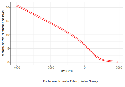
A note should be made that the Ørland curve was originally published with reference to the highest astronomical tide in the region (see Romundset and Lakeman 2019:66). To adjust this to mean sea-level, the difference in elevation between the highest astronomical tide and the mean sea-level has been been subtracted from the elevation values.
Furthermore, while variable uplift rates are also relevant for this
area, this is not corrected for in this example. The example therefore
focuses on the small area for which the curve was developed, where it
can be assumed to be directly applicable. Functionality to adjust for
variable displacement rates with shoredate is only accommodated
for the Skagerrak area through the function
interpolate_curve(). Thus, if similar adjustments are to
made in other areas, this will at present therefore have to be done
independently of shoredate, to which the adjusted curves can
then be passed.
Creating maps of Ørland
Having loaded the displacement curve, this can then be directly used
to shoreline date sites in locations where it applies, provided the
elevation of the sites above present sea-level is known. First we will
create a couple of fictitious site examples, each represented by a
point, and maps of their location to demonstrate the extendibility of
the target_plot() function.
# Create example sites
target_points <-  st_sfc(st_point(c(532719, 7065723)),
                         st_point(c(532896, 7066260)))

# Set CRS
target_points <- st_as_sf(target_points, crs = 32632)

# Add site names
target_points$name <- c("Example 1", "Example 2")
To create a map of where Ørland and these target points are located,
one can adapt the target_plot() function. First, set up the
geometries to be plotted:
# Load in the limit of the spatial coverage in south-eastern Norway,
# which is provided with the package
senorway <- st_read(system.file("extdata/spatial_limit.gpkg",
                                    package = "shoredate"), quiet = TRUE)

# Assign a name to this for the map legend
senorway$name <- "Skagerrak limit"

# Retrieve the first of the example points, to represent Ørland
orland <- target_points[1,]
orland$location = "Ørland"
Once this has been done we can use target_plot() to set
up a plot. Setting naturalearth_basemap to TRUE downloads a
world map from https://www.naturalearthdata.com/ using the
rnaturalearth package. This is stored in a temporary folder
and is deleted when the current R session is ended. The argument
naturalearth_zoom specifies the amount of cropping that is
done on this world map, with the provided targets as the focal point.
The argument crs_epsg is here the same as the default, but
is explicitly called to highlight that different coordinate reference
systems can be used. Setting the argument isobases to NA
means that the default isobases pertaining to south-eastern Norway are
excluded from the plot. Finally, setting target_labels to
FALSE excludes the labelling of the target points in the plot, which
will instead be handled with a legend in the code to follow below.
overview_map <- target_plot(targets = orland,
                      naturalearth_basemap = TRUE,
                      naturalearth_zoom = c(1000000, 1000000),
                      crs_epsg = 32632,
                      base_col = "black",
                      base_fill = "grey85",
                      isobases = NA,
                      target_labels =  FALSE)
## Reading layer `ne_10m_admin_0_countries' from data source `/tmp/RtmpzBrT1V/ne_10m_admin_0_countries.shp' using driver `ESRI Shapefile'
## Simple feature collection with 258 features and 168 fields
## Geometry type: MULTIPOLYGON
## Dimension: XY
## Bounding box: xmin: -180 ymin: -90 xmax: 180 ymax: 83.6341
## Geodetic CRS: WGS 84Having created a base plot, this can now be manipulated using other
functions from the package ggplot2.
overview_map <- overview_map +
        geom_sf(data = senorway, aes(col = name), fill = NA,
                   lwd = 0.5, show.legend = "polygon") +
        # Replotting the point for Ørland to add it to the legend
        geom_sf(data = orland, aes(fill = location),
                   col = "black", shape = 21,
                   size = 3, show.legend = "point") +
        scale_fill_manual(values = c("Ørland" = "red")) +
        scale_colour_manual(values = c("Skagerrak limit" = "red"),
                               guide = guide_legend(
                                          override.aes = list(shape = NA))) +
        theme(legend.position = "bottom",
              legend.title = element_blank()) +
        ggtitle(paste("Location of Ørland relative to the",
                       "spatial limit in south-eastern Norway"))
When the map displaying the location of Ørland is created, we can create a second map that shows the location of the example points, zoomed in at Ørland, which is located at the tip of the Fosen peninsula. While the map is fairly simple, it can nonetheless be useful to perform this exercise to make sure everything looks as it should.
# Create basemap
examples_map <- target_plot(targets = target_points,
                      naturalearth_basemap = TRUE,
                      naturalearth_zoom = c(15000, 10000),
                      base_col = "black",
                      base_fill = "grey85",
                      isobases = NA)

# Add axis labels and ticks, which are not returned with target_plot()
examples_map <- examples_map +
      theme(
        axis.text.y = element_text(),
        axis.text.x = element_text(),
        axis.ticks = element_line()) +
      coord_sf(datum = st_crs(target_points), expand = FALSE) +
      ggtitle("Location of example points in Ørland")

# Call overview map
overview_map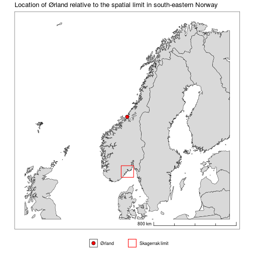
# Call map displaying the location of the example points
examples_map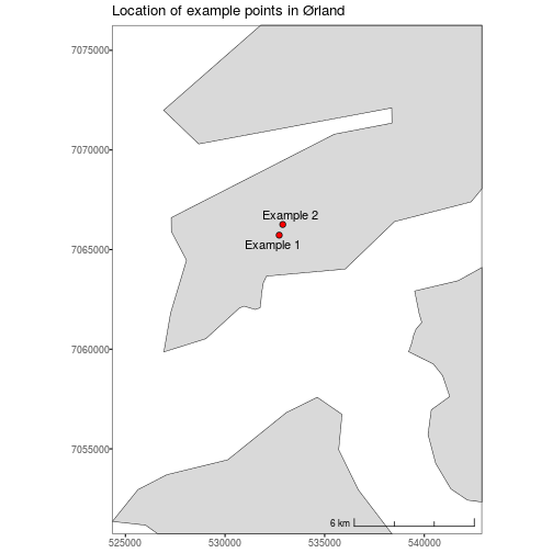
Dating example sites in Ørland
For this example, a raster retrieved from Amazon Web Service Terrain Tiles is used for finding the elevation of the example sites. This follows the procedure that is outlined in the main vignette.
# Retrieve raster
target_wgs84 <- st_transform(target_points, crs = 4326)
elev_raster <- elevatr::get_elev_raster(target_wgs84, z = 14,
                                        verbose = FALSE, src = "aws")
elev_raster <- terra::project(terra::rast(elev_raster), "epsg:32632")

# Plot the raster and sites for inspection
terra::plot(elev_raster)
plot(target_points, col = "black", add = TRUE)
text(st_coordinates(target_points) - 50, labels = target_points$name)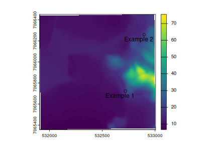
After the raster has been loaded we can find the elevation of the sites:
## [1] 17.74340 19.53946This elevation is retrieved by shoreline_date() if the
raster is passed to its elevation argument and the sites to
be dated are provided as spatial geometries. However, to illustrate the
point that all that is needed to use shoreline_date() is a
displacement curve and knowledge of these elevations, the function is
here called by only providing the displacement curve and providing a
character vector with the name of the sites and a numerical vector with
their elevations:
target_dates <- shoreline_date(sites = c("Example 1", "Example 2"),
                               target_curve = orland_disp,
                               elevation = c(17.7, 19.5))

# Plot the results
shoredate_plot(target_dates, multiplot = TRUE)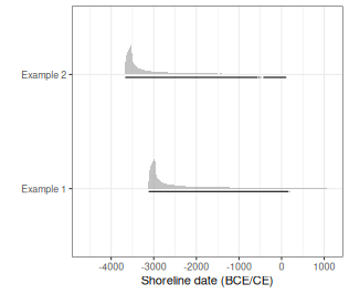
Finding the earliest possible date
As mentioned, the above implementation assumes that the relationship
between the sites and the shoreline is characterised by the same gamma
function as that identified for sites in south-eastern Norway. At
present, the only adjustment that is possible to do to this assumed
relationship is changing the parameters for the gamma function when
calling shoreline_date(), using the argument
model_parameters.
However, as an alternative it is also possible to perform the dating
procedure without accounting for any distance between the site and the
contemporaneous shoreline. This is done by setting the parameter
model to “none” when calling shoreline_date().
This thus effectively provides a termnius post quem date, under
the assumption that the earliest possible date for when the site was in
use is when the location of the site emerged from the sea.
While a terminus post quem date limits the further inferential steps that can be taken, it might be more appropriate to apply shoreline dating in this manner in regions where the relationship between sites and the shoreline is unknown. This can potentially also be extended to the dating of other phenomena such as rock art, or other cases where this relationship is less certain (see e.g. Sognnes 2003).
Furthermore, it could also be possible to reverse this logic in regions that have instead been subject to relative sea-level rise, where the date for when a location was inundated can provide a terminus ante quem date – the latest possible date for the use of a site. However, implementation of shoredate to regions which have experienced continuous or disjoint phases of relative sea-level rise remains to be developed.
# Finding the earliest possible date for the first example point
earliest_date <- shoreline_date(target_points[1,],
                                target_curve = orland_disp,
                                elevation = elev_raster,
                                model = "none",
                                hdr_prob = 1)

# Call to plot
shoredate_plot(earliest_date, site_name = TRUE)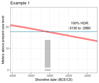
References
Roalkvam, I. 2023 A simulation-based assessment of the relation between Stone Age sites and relative sea-level change along the Norwegian Skagerrak coast. Quaternary Science Reviews 299:107880. DOI: 10.1016/j.quascirev.2022.107880
Romundset, A. and Lakeman, T.R. 2019. Shoreline displacement at Ørland since 6000 cal. yr BP. In Environment and Settlement: Ørland 600 BC – AD 1250: Archaeological Excavations at Vik, Ørland Main Air Base, edited by Ystgaard, I. Cappelen Damm Akademisk, Oslo, pp. 51–67. DOI: 10.23865/noasp.89
Sognnes, K. 2003. On Shoreline Dating of Rock Art. Acta Archaeologica 74:189–209. DOI: 10.1111/j.0065-001X.2003.aar740104.x